Galton Board

At the end of the 19th century, the English polymath Sir Francis C. Galton (1822–1911) developed an arrangement to demonstrate the so-called binomial distribution. This arrangement was later called the Galton board in his honour. A version of this has been realised in ADVENTURE LAND MATHEMATICS:

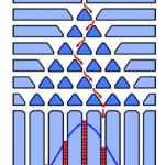
Between two glass plates, several 50-cent coins are fixed with three pins each and arranged evenly so that — as an overall structure — an equilateral triangle of twelve “cascades” results (see figure 1 below):

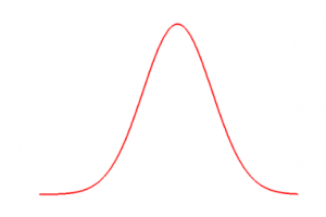
If you now let a coin fall in vertically from above, each of these obstacles (i.e. the locked 50-cent coins) randomly decides whether it falls to the right or to the left. The probability of this is $p=0.5$ in each case. Below the Galton board are several compartments in which the inserted coins are stacked on top of each other. That is, in this way a kind of bar chart is created that approximates the density of a normal distribution as the number of inserted coins increases. The shape of this density is a bell-shaped curve (“Gaussian bell curve“), as shown in the following figure 2:

1-cent, 2-cent, … or 50-cent coins are suitable for carrying out the experiment in ADVENTURE LAND MATHEMATICS.

Note: The coins thrown in for an experiment on the Galton board will later be used as a contribution to the work of the non-profit(!) association for the promotion of the work of ADVENTURE LAND MATHEMATICS. This is how the name “Geldtonbrett” came about for this exhibit.

And now … the mathematics:

The Galton board in ADVENTURE LAND MATHEMATICS has a total of $N=12$ steps, i.e. the inserted coin has to “choose” right or left exactly twelve times on its way down. It is reasonable to assume that all these decisions are stochastically independent of each other: Whether the coin decides one way or the other at an obstacle — it does not affect its behaviour below. So essentially the same random experiment is run twelve times in a row. So accordingly there is exactly

$2\cdot2\cdot2\cdot2\cdot2\cdot2\cdot2\cdot2\cdot2\cdot2\cdot2=2^{12}d= 4.096$

Ways in which the coin can behave. Each of these possibilities corresponds to exactly one path in the associated tree diagram. However, the experiment does not count how often a ball uses each of these (equally probable) paths, but how often it chooses right and left.

For this purpose, below the Galton board $N+1=13$ are compartments $F_0, F_1,\dots, F_{12}$ reflecting this. The coin lands in the compartment $F_n$ exactly when it decides exactly $n$ times for the right (and accordingly $(N-n)=(13-n)$ times for the left).

If one now conducts this experiment with a sufficiently large number of coins, it can be observed that most of them collect in the middle compartments. The outside compartments, on the other hand, are rarely reached.

This in turn has a simple mathematical reason: The number of paths that lead into the compartment $F_n$ is exactly ${N \choose n}={12 \choose n}$ , because it is necessary to select exactly $n$ of the $N=12$ steps where the coin decides to go right. Accordingly, the probability of ending up in compartment $F_n$ is exactly

$p_N(n) ={N \choose n}\cdot p^n\cdot(1-p)^{N-n}={N \choose n}2^{-N}={N \choose n}2^{-12}$

where $n=0,\ldots,12$ .

This probability distribution is called a binomial distribution with the parameters $p= 0.5$ (the probability of a coin falling to the right at an obstacle) and $N=12$ (the number of stages of the random experiment). The $p_N(n)$ are also called their individual probabilities.

The fact that the binomial distribution for “large” values $N$ is approximated by the normal distribution — i.e. is approximated — i.e. approximated — by the normal distribution, describes the so-called limit theorem of Moivre-Laplace:

$\sum_{n:a\leq\frac{n-\mu}{\sigma}\leq b}{p_N(n)}\to\frac{1}{\sqrt{2\pi}}\int_a^b{e^{-z^2/2}}dz$

for $N\to\infty$ , $a,b\in\mathbb R$ fixed and arbitrary, $\mu=Np$ and $\sigma=\sqrt{Np(1-p)}$ .

In the following, we sketch another proof of this theorem:

First, one observes that the density function

$z\mapsto f(z)=\frac{e^{-z^2/2}}{\sqrt{2\pi}}$

has the derivative $-zf(z)$ , i.e. satisfies the differential equation $f'(z)=-z f(z)$ . If we add that the integral

$\int_{-\infty}^\infty f(z)dz=1$

then the density function of the standard normal distribution

$f(z)=\frac{e^{-z^2/2}}{\sqrt{2\pi}}$

is obtained as a unique solution to this differential equation. The assertion of Moivre-Laplace’s limit theorem is now that the (suitably rescaled) “density function” of the binomial distribution with parameters $p$ and $N$ converges against this function $f(z)$ . By “rescale” we mean here that the $x$ coordinate is first shifted to the left by $\mu=pN$ and then the $x$ axis is compressed by $\sigma=\sqrt{Np(1-p)}$ and the $y$ axis is stretched by $\sigma$ . We thus obtain from the binomial distributed random variable $B_{N,p}$ with values in $\{0,\ldots,N\}$ , the random variable $B'_{N,p}$ which has values in

$\left\{\frac{-Np}{\sqrt{Np(1-p)}},\ldots,\frac{N(1-p)}{\sqrt{Np(1-p)}}\right\}.$

This is a discrete random variable with distribution

$\sum_{k=0}^N p_N(k)\delta_{\frac{k-\mu}{\sigma}},$

where $\delta_x$ is the Dirac measure in $x\in\mathbb R$ . Since the random variable $B'_{N,p}$ is discrete, it has no density function in the true sense. But we can replace the Dirac measure $\delta_x$ in the formula just noted by a measure of mass one $\lambda_x=\sigma\lambda\rvert_{[x-1/(2\sigma),x+1/(2\sigma)]}$ (where $\lambda$ denotes the Lebesgue measure) equally distributed on $[x-\sigma/2,x+\sigma/2]$ . In this way we obtain another random variable $B''_{N,p}$ , which has a density function. It is easy to see that the distributions of $B'_{N,p}$ and $B''_{N,p}$ are weakly equivalent in the limit, i.e. their difference converges weakly to $0$ for $N\to\infty$ . So we can work with $B''_{N,p}$ instead of $B'_{N,p}$ . To show that their distribution function weakly tends to $f\lambda$ ( $\lambda$ the Lebesgue measure), we now simply show that it satisfies the above differential equation $f'(z)=-zf(z)$ in the limit. So let us write $f_0$ for the density function of $B''_{N,p}$ and assume that $z=\frac{k-\mu}{\sigma}$ for a $k\in\{0,\ldots,N\}$ . This certainly makes sense, since such values fill the whole axis with increasing $N$ and lie ever closer together. Then we have

$-z=-\frac{k-\mu}{\sigma}$

and

$f_0(z)=\sigma p_N(k).$

But what is $f_0'(z)$ . In fact, $f_0$ is constant in an environment of $z$ , so $f_0'(z)=0$ should actually apply. But at the distance $1/(2\sigma)$ from $z$ $f_0$ suddenly makes a jump; so there $\lvert f_0'(z)\rvert=\infty$ would be. To account for both, we use a difference quotient instead of a differential quotient:

$f_0'(z)\approx\frac{f_0(z+1/\sigma)-f_0(z)}{1/\sigma}=\frac{\sigma p_N(k+1)-\sigma p_N(k)}{1/\sigma}=\sigma^2(p_N(k+1)-p_N(k)).\quad(\ast)$

Thus, for the left-hand side of the differential equation

$f_0'(z)=\sigma^2(p_N(k+1)-p_N(k))$

we obtain

and for the right-hand side

$-zf_0(z)=-\frac{k-\mu}{\sigma}\sigma p_N(k)=-(k-\mu)p_N(k)\quad(\ast).$

So, to check the above differential equation in the limit, it suffices — taking into account $(\ast)$ and $(\ast\ast)$ — to prove the equation

$-\frac{f_0'(z)}{zf_0(z)}=-\frac{p_N(k+1)-p_N(k)}{p_N(k)}\cdot\frac{\sigma^2}{k-\mu}\to 1$

for $N\to\infty$ . We leave this calculation to the reader and refer to the proof on Wikipedia where it is carried out. Since also $\int_{-\infty}^\infty f_0(z)dz=1$ , we are done. Of course, this sketch is not a rigorous proof — but it can be transformed into one with some effort.

Literature

[1] Henze, N.: Stochastik für Einsteiger. Eine Einführung in die faszinierende Welt des Zufalls, Springer Spektrum, 10. Auflage, Wiesbaden, 2013.

[2] https://en.wikipedia.org/wiki/De_Moivre%E2%80%93Laplace_theorem.