Skip to the content
  • Search
    • Deutsch
    • Leichte Sprache
    • Čeština
  • Font/Contrast
    • Change contrast
    • Enlarge font
  • Exhibition
    • The Exhibits
    • Mobile Adventure Land
    • MathsLive
  • Visit
    • Visitor information
    • Contact
  • Adventureland Online
    • Advanced Texts
    • Workshops2Go
    • #enjoyinglearning
  • Schools visiting
    • Schools visiting
    • Workshops
    • Tips for the visit
  • Leisure
    • Leisure
    • The Epsilon
    • Actionsbounds
    • Mathematics in Conversation
    • Handicraft sheets
    • Borderless Adventure Land
  • About Us
    • About Us
    • Support Association
    • Sponsors and Supporters
    • Jobs
    • Contact
  • Search
  • Font/Contrast
    • Kontrast ändern
    • Schrift vergrößern
    • Deutsch
    • Leichte Sprache
    • Čeština

Round trips through Saxony

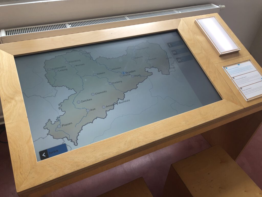
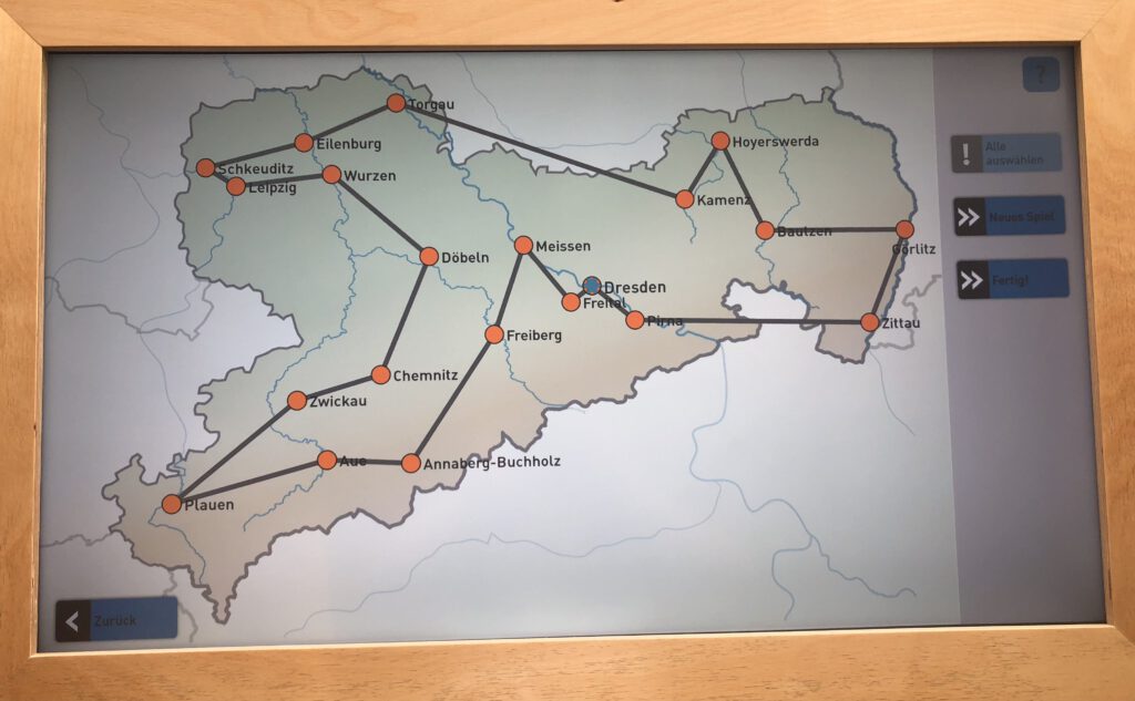
Imagine you are planning a round trip through the largest cities in Saxony. You only want to visit each city once and the round trip should be as short as possible. The “Round trip through Saxony” exhibit allows you to plan your journey as efficiently as possible.

Figure 1: The exhibit

And now … the mathematics:

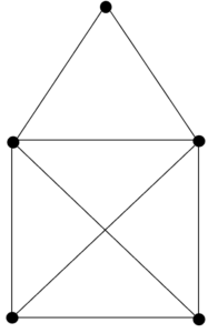
Such a problem is also called the “Traveling Salesmen Problem“ (TSP). This can be modeled using graphs. An (undirected) graph is an entity that consists of vertices and edges. Each edge connects two vertices (cf. [1]). For example, the “House of St Nicholas” is a graph consisting of 5 corners and 8 edges (see also the exhibit “Euler’s lines”).

Abbildung 2: House of St Nicholas
 In mathematics, we write this as follows: A graph (V,E) consists of
  • a finite set V of vertices,
  • a set E \subseteq \{ \{i,j\} \colon i,j \in V \} of edges.
Abbildung 3: Example of a graph

In addition, we assign each edge \{i,j\} \in E a quantity c_{ij} \geq 0, the so-called edge weight. This can be interpreted, for example, as a geographical length, as the time required to travel from i to j or as the cost of a journey.

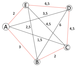
Figure 2 shows a graph whose corner set consists of the corners A,B,C,D,E and which has the edge set

    \begin{align*}E = \{ \{A,B\}, \{A,D\}, \{C,A\}, \{B,E\}, \{B,D\}, \{B,C\}, \{C,D\}, \{C,E\}, \{D,E\}, \{E,A\} \}.\end{align*}

Here, particularly, we do not distinguish the edges \{A,B\} and \{B,A\}, since c_{AB} = 4 = c_{BA} coincides. A graph with this property is also referred to as an undirected graph. In particular, the edge weights fulfill the triangle inequality, i.e. the distance between two vertices i and j, for example, is smaller than the distance from i to k plus the distance from k to j. In general, this can be written for any vertices i,j,k \in V as follows

    \begin{align*}c_{ij} \leq c_{ik} + c_{kj}.\end{align*}

The aim of a TSP is now to find the shortest tour (also called Hamilton circle) in the underlying graph, i.e. a round trip in which we visit each city only once and end in the city in which we started our journey. A tour is also called a circle in the graph, although it does not have to be circular. In Figure 3, for example, the red-coloured edges form a tour in this graph. Its length is then calculated by adding the edge weights, i.e. the length of this tour is

    \begin{align*}c_{AB} + c_{BC} + c_{CD} + c_{DE} + c_{EA} = 18.\end{align*}

However, there is a tour that is even shorter. Can you find it?

Modelling the exhibit as a graph

The graph modelling our exhibit has the corner set

    \begin{align*}V = \ &\{\text{Dresden, Leipzig, Chemnitz, Schkeuditz}, \text{ Eilenburg, Wurzen, Torgau, Döbeln}, \\ &\text{Plauen, Zwickau, Aue, Annaberg-Buchholz, Freiberg, Freital, Pirna, } \\ &\text{Meissen, Bautzen, Kamenz, } \text{Hoyerswerda, Görlitz, Zittau} \}.\end{align*}

It therefore consists of a total of 21 different cities, each of which represents a corner in our graph. The set of edges results from the choice of route through the cities of Saxony. For example, if we start our journey in Dresden and want to travel from there to Leipzig first, then this route would correspond to the edge

    \begin{align*}u \coloneqq \{ \text{Dresden, Leipzig} \} \in E.\end{align*}

The edge weight c_{Dresden, Leipzig} is the geographical distance between Dresden and Leipzig (“as the crow flies”).
Perhaps you were able to quickly determine the shortest route in the graph in Figure 2. However, as you will soon realise, this task is not so easy with this exhibit. This is because you have a total of

    \begin{align*}\frac{20!}{2} = 1 \, 216 \, 451 \, 004 \, 088 \, 320 \, 000\end{align*}

(i.e. over a trillion!) different tours available. Incidentally, the number of possible routes in the graph in Figure 2 is 12. As you can see, this number can increase significantly with a large number of corners. We will explain why this is the case in the next section.

P versus NP

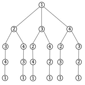
Let’s assume we want to visit n (n > 2) cities and we are already in one of these cities. From our starting point, we have exactly n - 1 other cities to choose from as our next destination. After choosing the second destination, we now have exactly n - 2 other cities to choose from for the third city, and so on. Combinatorially, we could say that we have an urn model without putting back, whereby we attach importance to the order. If we continue like this, we will have visited all n cities at some point. There is exactly one more station left, namely to return to our starting city. This results in an n + 1 step tree diagram.

Abbildung 4: {Tree diagram for n = 4

Figure 4 shows this for the case n = 4. Here you can also see that all routes occur twice, depending on the direction in which the tour is run (clockwise or anti-clockwise). For example, the tour 1 - 2 - 3 - 4 - 1 is the same as 1 - 4 - 3 - 2 - 1. There are therefore a total of

(1)   \begin{align*}\frac{1}{2} \cdot (n - 1) \cdot (n - 2) \cdots 1 = \frac{(n - 1)!}{2} \end{align*}

possible different tours available, where we multiply by \frac{1}{2} because, as just noted, each tour occurs twice. Incidentally, the number can also be obtained by counting and halving the number of all paths in the tree diagram.

If you now want to use a computer to determine the shortest tour, it would have to calculate every single tour and select the shortest one from all these tours. For large n this is no longer “efficient” and would take too long (certainly longer than a human life). According to (1), the number of calculation steps required for this even increases more than exponentially with the number of cities. However, it can always be decided quickly whether a selected edge set is also a tour in the graph, because a computer would only have to check whether we have ended our journey where we started it and whether every other city has only been visited once. This task can therefore be decided “efficiently” or in “polynomial time” by a computer, i.e. the number of calculation steps to check the correctness of a route depends at most polynomially on the number of corners. A possible, but not optimal, route can be seen in Figure 2.

Abbildung 5: A possible, but not optimal, solution for the TSP

There is also a scale on the exhibit that shows you how short your tour is compared to the optimum tour.

It is also said that the travelling salesman problem is in the complexity class NP (non-deterministic polynomial) and the decision problem, which determines whether a selected edge set is a tour, is in the complexity class P (polynomial). An unsolved problem to date is whether NP = P holds, i.e. whether the class P of all problems that can be solved in polynomial time is equal to the class NP of all problems for which a proposed solution can be checked for correctness in polynomial time. This problem is one of the seven Millennium Prize Problems, of which only the Poincaré conjecture was proved by Grigori Perelmann in 2002. In order to solve the P-NP problem, one would have to find an algorithm that can solve a problem from the complexity class NP in polynomial time. Since no one has yet succeeded in doing so, the majority of scientists assume that P \neq NP. In concrete terms, a proof of the P-NP problem would mean that a computer can “efficiently” calculate, for example, the shortest tour in a TSP in a short time. However, a proof could also have negative consequences, e.g. in encryption technology. If P = NP were to apply, there would be the possibility that encryption systems could be cracked in a very short time. As a result, banks’ security systems, among others, could be easily breached and our banking data would no longer be secure.

Literature

[1] Nitzsche, Manfred: Graphen für Einsteiger. Springer, 2005

[2] https://www.spektrum.de/news/loesung-fuer-p-np-problem/1494941

[3] https://en.wikipedia.org/wiki/Travelling_salesman_problem

[4] https://en.wikipedia.org/wiki/P_versus_NP_problem 

Opening Hours and Ticket Prices

Tuesday – Friday: 9 am – 5 pm
Saturday, Sunday and holidays: 10 am – 6 pm

Entry: 5 Euro / discount. 4 Euro

Special prices apply for groups and families, for guided tours or for photo and video permission.

  • Legal Notes
  • Data protection
  • Accessibility
© 2022

Adress

Erlebnisland Mathematik
Technische Sammlungen Dresden
Junghansstraße 1-3
01277 Dresden

Visitor Service

0351 – 488 7272 | service@museen-dresden.de